Least-Squares Line Fits and Associated Uncertainty

By David Archer

 

Introduction

 

There are several measurement situation where one is trying to determine if there is a linear relationship between a pair of measured values. For instance the relationship between stress and strain, voltage and current, input voltage and output voltage, etc.. In this article the basics of least-squares line fits will be discussed, along with a basic uncertainty analysis.

 

The General Least-Squares Problem

 

In the general least-squares problem, one has a set of measured data collected as ordered pairs

 

 

and one wants to fit this data to the functional form

 

 

where the c_i are parameters M parameters that define the function.

 

One can define the residuals of the data set from

 

 

which measures how far each data point deviates from the function along a vertical line. A measure of the goodness of the fit is the root-mean-square (RMS) value of the residuals

 

.

 

The general least-squares problem is to find the constants c_i that minimizes the RMS value of the residuals. From basic calculus, one knows one has a minimum if

 

 

One generates a series of M such equations for the M unknowns in the functional form. Solving this system of equations results in the least-squares fit for the particular functional form.

 

The Least-Squares Line Fit Problem

 

The problem at hand is to fit the data to the functional form

 

 

where the slope m, and the intercept b, are chosen to minimize the RMS residuals

 

.

 

Taking the derivative of this expression with respect to b and equating it to zero results in

 

.

 

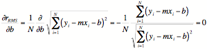With a little manipulation this reduces to

 

 

Performing the same operation for the parameter m,

 

 

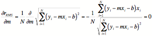
which can be manipulated into the form

 

 

To simplify these equations, the following quantities are introduced

 

 

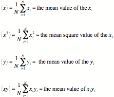
The equations that determine the minimum RMS residual can now be recast in the form

 

 

or written as a matrix equation

 

 

This system of equations have the solution

 

 

which solves the least squares problem.

 

Uncertainty Analysis

 

Assuming for the moment that the slope or intercept were the quantities that one was actually trying to measure, one should perform an uncertainty analysis on these parameters by using the  "Law of propagation of uncertainty" to determine the uncertainty in the slope and intercept in terms of the uncertainty in the measurement data.

 

The uncertainty in the slope  can be written

 

 

where  is the uncertainty associated with , and  is the uncertainty associated with .

 

It can be shown that the partial derivatives are

 

 

 

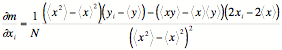
and

 

.

 

Similarly for the uncertainty in the intercept  is

 

 

and the partial derivatives are

 

 

and

 

.

 

Now it may also be the case that one wants to use the best fit line parameters to use in future measurements. In such cases one wants for a specific x

 

 

the uncertainty in the value y is then

 

 

Now what has been calculated to this point has been uncertainty associated with the fit itself. It assumes that the underlying phenomenon is linear. This may not be the case. However, one does have a quantity that is a direct measure of the "goodness" of the linearity assumption, namely the residuals.

 

There will be non-zero residuals for a given fit, even if the underlying phenomenon is perfectly linear, due to the uncertainty in the measurement. That however is predictable. The estimated residuals due to the measurement uncertainty is

 

 

This can be compared against the actual residuals. If the actual residuals are significantly larger than the predicted residuals, one can say there is some non-linearity in the underlying phenomenon. In such a case one would probably want to combine the RMS residuals with the uncertainty in y for an overall uncertainty statement.

 

Conclusion

 

The basics of least-squares line fits was presented, along with a basic uncertainty analysis. Hopefully this article can be useful as a reference if your measurement requires some sort of least-squares line fit. There are many phenomenon, and situations in calibration and measurement, where such a fit is useful.